SSEPCompact.py

From Werner KRAUTH

Revision as of 12:31, 10 June 2024 Werner (Talk | contribs) ← Previous diff		Revision as of 12:36, 10 June 2024 Werner (Talk | contribs) Next diff →
Line 1:		Line 1:
		+	==Context==
		+	This page is part of my [[BegRohu_Lectures_2024|2024 Beg Rohu Lectures]] on "The second Markov chain revolution" at the [https://www.ipht.fr/Meetings/BegRohu2024/index.html Summer School] "Concepts and Methods of Statistical Physics" (3 - 15 June 2024).
		+
	import math		import math
	import random		import random
Line 33:		Line 36:
	Text = 'Total time = ' + str(prefactor) + ' * N ^ ' + str(exponent) + ' * log N'		Text = 'Total time = ' + str(prefactor) + ' * N ^ ' + str(exponent) + ' * log N'
	print(' ' * (NSites// 2 + 1 - len(Text) // 2) + Text + ' ' * (NSites// 2 + 1 - len(Text) // 2))		print(' ' * (NSites// 2 + 1 - len(Text) // 2) + Text + ' ' * (NSites// 2 + 1 - len(Text) // 2))
		+
		+	==Output==
		+
		+	Here is output of the above Python program. The histogram is absolutely flat, without any corrections. But this is normal, given that the simulation has run, for each of the realizations of the random map, an infinite number of iterations.
		+
		+	[[Image:Backward position t0.png|left|600px|border|Coupling-from-the-past approach to sampling.]]
		+	<br clear="all" />
		+
		+	==Further Information==
		+
		+	==References==

---

Revision as of 12:36, 10 June 2024

Contents 1 Context 2 Output 3 Further Information 4 References

Context

This page is part of my 2024 Beg Rohu Lectures on "The second Markov chain revolution" at the Summer School "Concepts and Methods of Statistical Physics" (3 - 15 June 2024).

import math
import random
exponent = 3.0
alpha = 0.5
prefactor = 1.0
NPart = 64; NSites = 2 * NPart
NIter = int(prefactor * NPart ** exponent * math.log(NPart))
NStrob = NIter // 40
Conf = [1] * NPart + [0] * (NSites - NPart)
Active = random.randint (0, NSites - 1)
while Conf[Active] != 1:
    Active = random.randint(0, NSites - 1)
Text = 'Periodic SSEP, N= ' + str(NPart) + ', L= ' + str(NSites)
print(' ' * (NSites// 2 + 1 - len(Text) // 2) + Text + ' ' * (NSites// 2 + 1 - len(Text) // 2))
print('-' * (NSites + 2))
for iter in range(NIter):
    Active = random.randint (0, NSites - 1)
    while Conf[Active] != 1: Active = random.randint(0, NSites - 1)
    Step = random.choice([-1,1])
    NewActive = (Active + Step) % NSites
    if Conf[NewActive] == 0: Conf[Active], Conf[NewActive] = 0, 1
    PP = '|'
    ktot= 0
    for k in range(NSites):
        if Conf[k] == 0:
            PP += ' '
        else:
           ktot += 1
           if ktot != NPart / 2: PP += 'X'
           else: PP += '|'
    if iter % NStrob == 0: print(PP)
print('-' * (NSites + 2))
Text = 'Total time = ' + str(prefactor) +  ' *  N ^ ' + str(exponent) + ' * log N'
print(' ' * (NSites// 2 + 1 - len(Text) // 2) + Text + ' ' * (NSites// 2 + 1 - len(Text) // 2))

Output

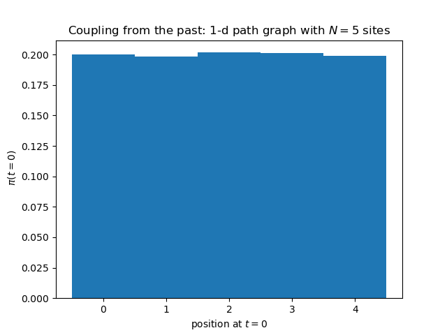
Here is output of the above Python program. The histogram is absolutely flat, without any corrections. But this is normal, given that the simulation has run, for each of the realizations of the random map, an infinite number of iterations.

Further Information

References