Diffusion CFTP.py
From Werner KRAUTH
| Revision as of 12:13, 6 June 2024 Werner (Talk | contribs) ← Previous diff |
Current revision Werner (Talk | contribs) (→Python program) |
||
| Line 1: | Line 1: | ||
| + | ==Context== | ||
| + | This page is part of my [[BegRohu_Lectures_2024|2024 Beg Rohu Lectures]] on "The second Markov chain revolution" at the [https://www.ipht.fr/Meetings/BegRohu2024/index.html Summer School] "Concepts and Methods of Statistical Physics" (3 - 15 June 2024). | ||
| + | |||
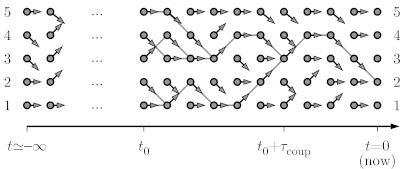
| + | The present program illustrates the coupling-from-the-past approach to Markov-chain sampling introduced by Propp and Wilson in 1997. This paper is definitely part of the ''second Revolution''. It illustrates how Markov-chain sampling can obtain samples from the stationary distribution, without any corrections whatsoever. As in the other program in the series started by [[Diffusion.py |Diffusion.py]], we consider a particle diffusing on a path graph with five sites, with "down", "up", and "straight¨ moves that are cropped at the boundaries (there are no periodic boundary conditions). We consider the formulation of a Markov chain in terms of random maps, but run from time t=-infinity up to time t=0. | ||
| + | |||
| + | [[Image:One d cftp.png|left|600px|border|Coupling-from-the-past approach to sampling.]] | ||
| + | <br clear="all" /> | ||
| + | At time t=-infinity, as shown, the pebble starts on configuration 1 so that, by time t=0, it has run for an infinite time. Whatever the mixing time and the relaxation time, by t=0, it must sample the stationary distribution (the uniform distribution on the five sites). The below program constructs just as many sets of arrows as needed to conclude where it finishes its infinitely long journey. | ||
| + | |||
| + | ==Python program== | ||
| + | |||
| import random | import random | ||
| import matplotlib.pyplot as plt | import matplotlib.pyplot as plt | ||
| Line 13: | Line 24: | ||
| if arrows[N - 1] == 1: arrows[N - 1] = 0 | if arrows[N - 1] == 1: arrows[N - 1] = 0 | ||
| all_arrows[time_tot] = arrows | all_arrows[time_tot] = arrows | ||
| - | positions=set(range(0, N)) | + | positions = set(range(0, N)) |
| for t in range(time_tot, 0): | for t in range(time_tot, 0): | ||
| positions = set([b + all_arrows[t][b] for b in positions]) | positions = set([b + all_arrows[t][b] for b in positions]) | ||
| Line 23: | Line 34: | ||
| plt.savefig('backward_position_t0.png') | plt.savefig('backward_position_t0.png') | ||
| plt.show() | plt.show() | ||
| + | |||
| + | Note that "arrows" is a list, and all_arrows a dictionary containing the arrows for each position (0,1,...,N - 1). This dictionary contains exactly the random map of arrows in the above picture, from time time_tot to time -1. | ||
| + | |||
| + | ==Output== | ||
| + | |||
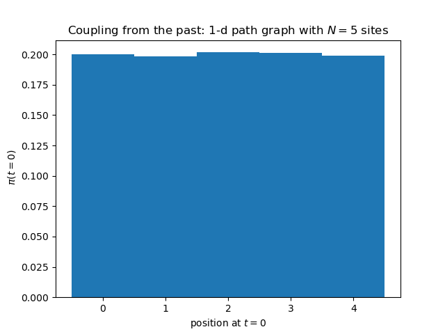
| + | Here is output of the above Python program. The histogram is absolutely flat, without any corrections. But this is normal, given that the simulation has run, for each of the realizations of the random map, an infinite number of iterations. | ||
| + | |||
| + | [[Image:Backward position t0.png|left|600px|border|Coupling-from-the-past approach to sampling.]] | ||
| + | <br clear="all" /> | ||
| + | |||
| + | ==Further Information== | ||
| + | |||
| + | * Rather than to run the simulation until t=0, one might be tempted to stop it as soon as the configurations have coupled at some time t < 0. This is tested in the following program, but it is wrong for obvious reasons: The goal was to infer the position at t=0 of a simulation that has run since time t=-infinity. | ||
| + | * The above program is easily adapted to a non-uniform stationary distribution pi(1),...,pi(N-1), and its output is then equivalent to what we would obtain using the direct-sampling algorithms that I discussed in BegRohu Lecture 1, first and foremost [[Walker.py| Walker's algorithm]]. However, Walker's algorithm always requires the stationary probabilities on the sample space to be evaluated and rearranged in some way, whereas the CFTP approach to Markov chains can be often applied for huge sample spaces, way larger than what can be listed. This is itself an astonishing story, that I hope to have time to relate in later lectures. | ||
| + | * A truly astonishing direct-sampling algorithm [[Stopping circle.py | Stopping_cycle.py]], based on the concept of strong stationary stopping times, is discussed in Lecture 5. However, this algorithm comes with a no-go theorem by Lovász and Winkler, that it is only correct for the cycle graph (the graph in the above example, but with periodic boundary conditions), and for the complete graph. | ||
| + | |||
| + | ==References== | ||
| + | |||
| + | |||
| + | The reference is: | ||
Current revision
Contents |
Context
This page is part of my 2024 Beg Rohu Lectures on "The second Markov chain revolution" at the Summer School "Concepts and Methods of Statistical Physics" (3 - 15 June 2024).
The present program illustrates the coupling-from-the-past approach to Markov-chain sampling introduced by Propp and Wilson in 1997. This paper is definitely part of the second Revolution. It illustrates how Markov-chain sampling can obtain samples from the stationary distribution, without any corrections whatsoever. As in the other program in the series started by Diffusion.py, we consider a particle diffusing on a path graph with five sites, with "down", "up", and "straight¨ moves that are cropped at the boundaries (there are no periodic boundary conditions). We consider the formulation of a Markov chain in terms of random maps, but run from time t=-infinity up to time t=0.
At time t=-infinity, as shown, the pebble starts on configuration 1 so that, by time t=0, it has run for an infinite time. Whatever the mixing time and the relaxation time, by t=0, it must sample the stationary distribution (the uniform distribution on the five sites). The below program constructs just as many sets of arrows as needed to conclude where it finishes its infinitely long journey.
Python program
import random
import matplotlib.pyplot as plt

N = 5
pos = []
for stat in range(100000):
   all_arrows = {}
   time_tot = 0
   while True:
      time_tot -= 1
      arrows = [random.choice([-1, 0, 1]) for i in range(N)]
      if arrows[0] == -1: arrows[0] = 0
      if arrows[N - 1] == 1: arrows[N - 1] = 0
      all_arrows[time_tot] = arrows
      positions = set(range(0, N))
      for t in range(time_tot, 0):
         positions = set([b + all_arrows[t][b] for b in positions])
      if len(positions) == 1: break
   a = positions.pop()
   pos.append(a)
plt.title('Backward coupling: 1-d with walls: position at t=0')
plt.hist(pos, bins=N, range=(-0.5, N - 0.5), density=True)
plt.savefig('backward_position_t0.png')
plt.show()
Note that "arrows" is a list, and all_arrows a dictionary containing the arrows for each position (0,1,...,N - 1). This dictionary contains exactly the random map of arrows in the above picture, from time time_tot to time -1.
Output
Here is output of the above Python program. The histogram is absolutely flat, without any corrections. But this is normal, given that the simulation has run, for each of the realizations of the random map, an infinite number of iterations.
Further Information
- Rather than to run the simulation until t=0, one might be tempted to stop it as soon as the configurations have coupled at some time t < 0. This is tested in the following program, but it is wrong for obvious reasons: The goal was to infer the position at t=0 of a simulation that has run since time t=-infinity.
- The above program is easily adapted to a non-uniform stationary distribution pi(1),...,pi(N-1), and its output is then equivalent to what we would obtain using the direct-sampling algorithms that I discussed in BegRohu Lecture 1, first and foremost Walker's algorithm. However, Walker's algorithm always requires the stationary probabilities on the sample space to be evaluated and rearranged in some way, whereas the CFTP approach to Markov chains can be often applied for huge sample spaces, way larger than what can be listed. This is itself an astonishing story, that I hope to have time to relate in later lectures.
- A truly astonishing direct-sampling algorithm Stopping_cycle.py, based on the concept of strong stationary stopping times, is discussed in Lecture 5. However, this algorithm comes with a no-go theorem by Lovász and Winkler, that it is only correct for the cycle graph (the graph in the above example, but with periodic boundary conditions), and for the complete graph.
References
The reference is:


