Diffusion CFTP.py
From Werner KRAUTH
(Difference between revisions)
| Revision as of 15:10, 6 June 2024 Werner (Talk | contribs) ← Previous diff |
Revision as of 15:03, 7 June 2024 Werner (Talk | contribs) Next diff → |
||
| Line 1: | Line 1: | ||
| ==Context== | ==Context== | ||
| This page is part of my [[BegRohu_Lectures_2024|2024 Beg Rohu Lectures]] on "The second Markov chain revolution" at the [https://www.ipht.fr/Meetings/BegRohu2024/index.html Summer School] "Concepts and Methods of Statistical Physics" (3 - 15 June 2024). | This page is part of my [[BegRohu_Lectures_2024|2024 Beg Rohu Lectures]] on "The second Markov chain revolution" at the [https://www.ipht.fr/Meetings/BegRohu2024/index.html Summer School] "Concepts and Methods of Statistical Physics" (3 - 15 June 2024). | ||
| + | |||
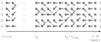
| + | In the example of a particle diffusing on a path graph with five sites, with moves from configuration i to [i-1, i, i] being proposed, we consider the formulation of a Markov chain in terms of random maps, but run from time t=-infinity up to time t=0. | ||
| + | |||
| + | [[Image:One d cftp.png|left|600px|border|Coupling-from-the-past approach to sampling.]] | ||
| + | <br clear="all" /> | ||
| ==Python program== | ==Python program== | ||
| Line 28: | Line 33: | ||
| plt.savefig('backward_position_t0.png') | plt.savefig('backward_position_t0.png') | ||
| plt.show() | plt.show() | ||
| + | |||
| + | ==Output== | ||
Revision as of 15:03, 7 June 2024
Context
This page is part of my 2024 Beg Rohu Lectures on "The second Markov chain revolution" at the Summer School "Concepts and Methods of Statistical Physics" (3 - 15 June 2024).
In the example of a particle diffusing on a path graph with five sites, with moves from configuration i to [i-1, i, i] being proposed, we consider the formulation of a Markov chain in terms of random maps, but run from time t=-infinity up to time t=0.
Python program
import random
import matplotlib.pyplot as plt

N = 5
pos = []
for stat in range(100000):
   all_arrows = {}
   time_tot = 0
   while True:
      time_tot -= 1
      arrows = [random.choice([-1, 0, 1]) for i in range(N)]
      if arrows[0] == -1: arrows[0] = 0
      if arrows[N - 1] == 1: arrows[N - 1] = 0
      all_arrows[time_tot] = arrows
      positions=set(range(0, N))
      for t in range(time_tot, 0):
         positions = set([b + all_arrows[t][b] for b in positions])
      if len(positions) == 1: break
   a = positions.pop()
   pos.append(a)
plt.title('Backward coupling: 1-d with walls: position at t=0')
plt.hist(pos, bins=N, range=(-0.5, N - 0.5), density=True)
plt.savefig('backward_position_t0.png')
plt.show()

