Diffusion.py

From Werner KRAUTH

Revision as of 09:22, 9 June 2024 Werner (Talk | contribs) (→Context) ← Previous diff		Revision as of 10:14, 9 June 2024 Werner (Talk | contribs) Next diff →
Line 3:		Line 3:
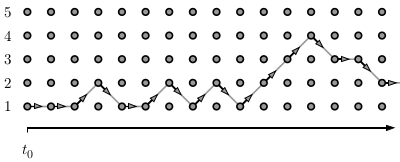
	We consider a particle diffusing on a path graph with five sites, always starting at position i = 0, at time t=0. Arrows go "down", "straight" and "up" with equal probability. In application of the Metropolis algorithm, an arrow that goes outside the range [0, N - 1] is rejected, that is, replaced by a straight arrow. The stationary distribution of this reversible Markov chain is uniform on the N sites, because the probability to move from site i to site j equals the probability to move from site j to site i.		We consider a particle diffusing on a path graph with five sites, always starting at position i = 0, at time t=0. Arrows go "down", "straight" and "up" with equal probability. In application of the Metropolis algorithm, an arrow that goes outside the range [0, N - 1] is rejected, that is, replaced by a straight arrow. The stationary distribution of this reversible Markov chain is uniform on the N sites, because the probability to move from site i to site j equals the probability to move from site j to site i.
		+
		+	[[Image:One d single.png|left|600px|border|Diffusion on a path graph with 5 sites.]]
		+	<br clear="all" />
	==Python program==		==Python program==
Line 29:		Line 32:
	==Further Information==		==Further Information==
-	Rather than to start at the 'bad' initial configuration i(t=0) = 0, one might be tempted to start it in the middle, but this contradicts the fact that, in real applications, one cannot usually choose a "good" initial configuration. One may also want to replace the 'bad' initial configuration by a random initial configuration i(t=0) = choice(0, ... N - 1). But this would mean that we do not have to do Markov-chain sampling at all, because a direct-sampling strategy is available. All this was discussed in detail in the lectures, and gave rise to lively discussions.	+	* Rather than to start at the 'bad' initial configuration i(t=0) = 0, one might be tempted to start it in the middle, but this contradicts the fact that, in real applications, one cannot usually choose a "good" initial configuration.
		+	* One may also want to replace the 'bad' initial configuration by a random initial configuration i(t=0) = choice(0, ... N - 1). But this would mean that we do not have to do Markov-chain sampling at all, because a direct-sampling strategy is available.
		+
		+	All this was discussed in detail in the lectures, and gave rise to lively discussions.

---

Revision as of 10:14, 9 June 2024

Contents 1 Context 2 Python program 3 Output 4 Further Information

Context

This page is part of my 2024 Beg Rohu Lectures on "The second Markov chain revolution" at the Summer School "Concepts and Methods of Statistical Physics" (3 - 15 June 2024).

We consider a particle diffusing on a path graph with five sites, always starting at position i = 0, at time t=0. Arrows go "down", "straight" and "up" with equal probability. In application of the Metropolis algorithm, an arrow that goes outside the range [0, N - 1] is rejected, that is, replaced by a straight arrow. The stationary distribution of this reversible Markov chain is uniform on the N sites, because the probability to move from site i to site j equals the probability to move from site j to site i.

Python program

import random
import matplotlib.pyplot as plt

N = 5
data = []
tmax = 10
for stat in range(100000):
   pos = 0
   for t in range(tmax):
      pos = min(max(pos + random.choice([-1, 0, 1]), 0), N - 1)
   data.append(pos)
plt.title('diffusion starting at $x=0$,  $t = $' + str(tmax))
plt.hist(data, bins=N, range=(-0.5, N-0.5), density=True)
plt.savefig('diffusion.png')
plt.show()

Output

Here is output of the above Python program. Although the stationary distribution is flat, as discussed above, the distribution pi^t, at finite times t is biased towards the initial configuration i(t=0) = 0. The below figure shows

Further Information

• Rather than to start at the 'bad' initial configuration i(t=0) = 0, one might be tempted to start it in the middle, but this contradicts the fact that, in real applications, one cannot usually choose a "good" initial configuration.
• One may also want to replace the 'bad' initial configuration by a random initial configuration i(t=0) = choice(0, ... N - 1). But this would mean that we do not have to do Markov-chain sampling at all, because a direct-sampling strategy is available.

All this was discussed in detail in the lectures, and gave rise to lively discussions.