Diffusion.py

From Werner KRAUTH

Revision as of 10:14, 9 June 2024 Werner (Talk | contribs) ← Previous diff		Revision as of 10:58, 9 June 2024 Werner (Talk | contribs) (→Python program) Next diff →
Line 24:		Line 24:
	plt.show()		plt.show()
		+	NB: The line containing the "pos = min(max ... " statement may appear cryptic, but it simply performs the random walk from the position "pos", with the necessary cutting at the boundaries in order to avoid that the random walk exits the range [0, N-1]
	==Output==		==Output==

---

Revision as of 10:58, 9 June 2024

Contents 1 Context 2 Python program 3 Output 4 Further Information

Context

This page is part of my 2024 Beg Rohu Lectures on "The second Markov chain revolution" at the Summer School "Concepts and Methods of Statistical Physics" (3 - 15 June 2024).

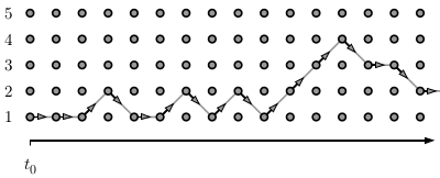
We consider a particle diffusing on a path graph with five sites, always starting at position i = 0, at time t=0. Arrows go "down", "straight" and "up" with equal probability. In application of the Metropolis algorithm, an arrow that goes outside the range [0, N - 1] is rejected, that is, replaced by a straight arrow. The stationary distribution of this reversible Markov chain is uniform on the N sites, because the probability to move from site i to site j equals the probability to move from site j to site i.

Python program

import random
import matplotlib.pyplot as plt

N = 5
data = []
tmax = 10
for stat in range(100000):
   pos = 0
   for t in range(tmax):
      pos = min(max(pos + random.choice([-1, 0, 1]), 0), N - 1)
   data.append(pos)
plt.title('diffusion starting at $x=0$,  $t = $' + str(tmax))
plt.hist(data, bins=N, range=(-0.5, N-0.5), density=True)
plt.savefig('diffusion.png')
plt.show()

NB: The line containing the "pos = min(max ... " statement may appear cryptic, but it simply performs the random walk from the position "pos", with the necessary cutting at the boundaries in order to avoid that the random walk exits the range [0, N-1]

Output

Here is output of the above Python program. Although the stationary distribution is flat, as discussed above, the distribution pi^t, at finite times t is biased towards the initial configuration i(t=0) = 0. The below figure shows

Further Information

• Rather than to start at the 'bad' initial configuration i(t=0) = 0, one might be tempted to start it in the middle, but this contradicts the fact that, in real applications, one cannot usually choose a "good" initial configuration.
• One may also want to replace the 'bad' initial configuration by a random initial configuration i(t=0) = choice(0, ... N - 1). But this would mean that we do not have to do Markov-chain sampling at all, because a direct-sampling strategy is available.

All this was discussed in detail in the lectures, and gave rise to lively discussions.