Diffusion CFTP.py

From Werner KRAUTH

Context

This page is part of my 2024 Beg Rohu Lectures on "The second Markov chain revolution" at the Summer School "Concepts and Methods of Statistical Physics" (3 - 15 June 2024).

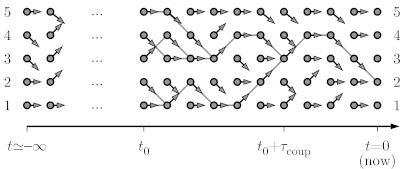
In the example of a particle diffusing on a path graph with five sites, with moves from configuration i to [i-1, i, i] being proposed, we consider the formulation of a Markov chain in terms of random maps, but run from time t=-infinity up to time t=0.

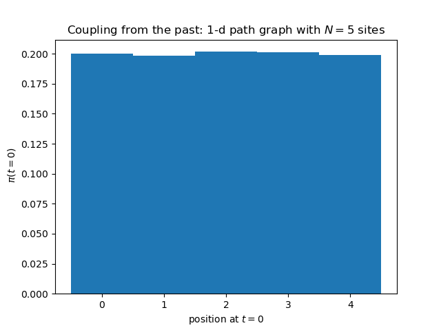
At time t=-infinity, as shown, the pebble starts on configuration 1, so that, by time t=0, it must sample the stationary distribution (the uniform distribution on the five sites). The below program constructs just as many set of arrows as needed to conclude on where it finishes it infinitely long journey.

Python program

import random
import matplotlib.pyplot as plt

N = 5
pos = []
for stat in range(100000):
   all_arrows = {}
   time_tot = 0
   while True:
      time_tot -= 1
      arrows = [random.choice([-1, 0, 1]) for i in range(N)]
      if arrows[0] == -1: arrows[0] = 0
      if arrows[N - 1] == 1: arrows[N - 1] = 0
      all_arrows[time_tot] = arrows
      positions=set(range(0, N))
      for t in range(time_tot, 0):
         positions = set([b + all_arrows[t][b] for b in positions])
      if len(positions) == 1: break
   a = positions.pop()
   pos.append(a)
plt.title('Backward coupling: 1-d with walls: position at t=0')
plt.hist(pos, bins=N, range=(-0.5, N - 0.5), density=True)
plt.savefig('backward_position_t0.png')
plt.show()

Output