 |
(1) |
|
(1) |
 |
(2) |
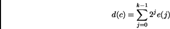
As an example, we code the 16 boolean automata with two inputs from 0 to 15. We choose as the most significant bit the one which corresponds to the input configuration 11 and as the least significant bit the one which corresponds to 00.
The AND function, for example, has a code of 8:
| (3) |
| (4) |
1. Knowing the inputs of each automaton.
In the general case, for an arbitrary connectivity, each input of each
automaton is given by a matrix: in the case of automata with two inputs,
two matrices, called for example ![]() and
and ![]() ,
define input #1 automaton and input #2 automaton for each of the automata.
,
define input #1 automaton and input #2 automaton for each of the automata.
For the example of figure 2.4:
| (5) | |||
| (6) | |||
| (7) | |||
| (8) |
In general, it is not necessary to define the outputs of each automaton.
In the case of cellular connectivity, it can be simpler to recalculate the input automata each time rather than to store them in memory.
2. The choice of the transition rules of the automata.
In the case of boolean automata, the result of the transition rule must
be given for each automaton and for each input configuration. We then use
a matrix with subscripts ![]() and
and ![]() ,
where one subscript refers to the automaton and the other to the input
configuration. This second subscript is the decimal code of the input configuration,
incremented by 1. For two inputs:
,
where one subscript refers to the automaton and the other to the input
configuration. This second subscript is the decimal code of the input configuration,
incremented by 1. For two inputs:
| (9) |
3. The choice of the mode of iteration (see the corresponding programming principle below).
2. The initial configuration of the network must be chosen. Depending on the application, it can be:
![]() programmed, for simple cases of a homogeneous configuration, or of a random
configuration. In the case of an exhaustive study to determine
the iteration
graph, the decimal code of the configuration is the index of the initial
condition loop.
programmed, for simple cases of a homogeneous configuration, or of a random
configuration. In the case of an exhaustive study to determine
the iteration
graph, the decimal code of the configuration is the index of the initial
condition loop.
![]() input from the keyboard, using a text editor or a graphical program.
input from the keyboard, using a text editor or a graphical program.
![]() or finally, it can be determined by external data gathered by a set of
sensors, in the case of an application to image recognition or more generally
to patterns.
or finally, it can be determined by external data gathered by a set of
sensors, in the case of an application to image recognition or more generally
to patterns.
| (10) |
![]() for iteration in series, the state of the automaton is updated directly
and we proceed to evaluate the following automaton. The preceding equation
can therefore be written:
for iteration in series, the state of the automaton is updated directly
and we proceed to evaluate the following automaton. The preceding equation
can therefore be written:
| (11) |
| (12) |
We initially set the color of the matrix to 0. Starting from the first configuration, we iterate the state change functions, placing 1's in the elements of the vector graph which correspond to the nodes which have been reached. Of course, we look at the state of each node before changing it: if it is equal to 1, the limit cycle has been reached.
The algorithm continues, incrementing the color of the nodes each time we look for a new basin, starting from the smallest configuration whose color is still 0. The iteration of the state change functions stops each time the color differs from 0: we have found a new basin of attraction if the color found is the same as that of the initial condition we started from. If the color is smaller, we are falling into a basin that has already been found. The preceding color must therefore be reassigned, starting from the last initial condition. The retrace operations are faster if we keep a successor matrix which stores the successor of each configuration. Similarly, during the retrace, one can increment a counter at each step to measure the periods.
The algorithm is finished when all of the nodes are colored. The highest color gives the number of attractors.
To find a limit cycle, a reference must be stored in memory: this is
the configuration reached by the network after an arbitrary time which
is assumed to be greater than the transient period. The algorithm consists
of taking the reference at time tref, and comparing it to all of the configurations
obtained. A counter can be used to measure the period. It is possible that
the reference may have been taken too soon: in fact the comparison is done
between times tref and 2![]() tref.
If the limit cycle has not been detected at 2
tref.
If the limit cycle has not been detected at 2![]() tref,
we take a new reference at 2
tref,
we take a new reference at 2![]() tref
and we multiply the search time by 2. The operation ``new reference-new
search'' continues until the limit cycle is reached, unless we decided
a priori to interrupt the search at a maximum time.
tref
and we multiply the search time by 2. The operation ``new reference-new
search'' continues until the limit cycle is reached, unless we decided
a priori to interrupt the search at a maximum time.
To estimate the number of attractors, we must compare the configurations reached during a limit cycle to the configurations obtained for a previously determined limit cycle. If number of attractors is high, this can be a long search. This is why certain decimal coding are sometimes used.
It is not necessary to keep connection matrices representing the inputs of the automata, since each matrix can generally be obtained by a simple translation from the position of the automaton under consideration. A small difficulty comes up due to the finite character of the lattice used in simulations. Cellular automata are defined for infinite lattices, whereas the simulated lattices are limited by boundaries. There are several ways of dealing with boundary effects. One way, for example, is to fix the states of the automata on the boundaries to arbitrary values. The most frequent solution used in simulations consists of connecting opposite edges to each other, which has the advantage of being less rigid than the previous solution. A linear lattice is then forms a circle, and a higher dimensional lattice forms a torus or a hypertorus.
To take into account the conditions at the edges, we add two ``surfaces''
inside the lattice (in fact, an automaton at each edge for one dimension,
two rows of automata in two dimensions, etc.). The iteration loops which
calculate
the new state, neta![]() ,
only apply to the internal lattice. The states of the edges are only updated
during the second loop, which updates the vector eta
,
only apply to the internal lattice. The states of the edges are only updated
during the second loop, which updates the vector eta![]() ;
and they then take on the values of the new eta calculated for the ``real''
edge to which they are connected. For example, if a linear lattice of 10
automata is being simulated, these automata are numbered from 2 to 11.
We add to them a left edge, numbered 1, and a right edge, numbered 12.
At the beginning of any loop from 2 to 11 to update neta
;
and they then take on the values of the new eta calculated for the ``real''
edge to which they are connected. For example, if a linear lattice of 10
automata is being simulated, these automata are numbered from 2 to 11.
We add to them a left edge, numbered 1, and a right edge, numbered 12.
At the beginning of any loop from 2 to 11 to update neta![]() ,
eta
,
eta![]() is equal to eta
is equal to eta![]() and eta
and eta![]() is equal to eta
is equal to eta![]() .
In this way, the state of automaton 11, the farthest to the right, is set
as function of a right-hand signal sent by automaton 2, which is the farthest
to the left. Of course, if the connections involve more than the nearest
neighbors, the size of the edges is correspondingly increased.
.
In this way, the state of automaton 11, the farthest to the right, is set
as function of a right-hand signal sent by automaton 2, which is the farthest
to the left. Of course, if the connections involve more than the nearest
neighbors, the size of the edges is correspondingly increased.
Regardless of the dimension of the lattice, each automaton can be referenced
by a single whole number. For a cube with dimensions ![]() ,
, ![]() ,
and
,
and ![]() ,
the subscript
,
the subscript ![]() of the automaton in a vector eta, for example, is then given by:
of the automaton in a vector eta, for example, is then given by:
| (13) |
| (14) |
If the lattice is one-dimensional, its successive different configurations can be displayed one after the other, according to Wolfram's representation. Rather than ``generating'' boring tables of 0's and 1's, it is more readable to code 0's by blanks or dots and 1's by plusses + or asterisks *. Word processing printers can sometimes cause problems if they print proportional characters: a constant spacing must be set so as to not scramble the output table. Of course, we can also choose a graphical mode of representation, which has sometimes been done in this book, representing the states of the automata by white or black dots.
If the lattice is two-dimensional, a powerful computer is needed to observe the output in ``real time,'' otherwise visually we can only see a sweep across the screen corresponding to the sequential update of the pixels. By using certain codes based on an alphanumeric representation, or on the color, we can integrate information about several time intervals within a single table (see figures 4.5 or 10.4).
Assume we want to find the minimum of ![]() ,
a function of a single variable:
,
a function of a single variable:
| (15) |
| (16) |
In the case of a function of several variables, ![]() ,
, ![]() ,
, ![]() ,...the
method can be generalized by using the gradient of
,...the
method can be generalized by using the gradient of ![]() .
The iteration formula then becomes:
.
The iteration formula then becomes:
| (17) | |||
| (18) | |||
| (19) |
The notation ![]() represents the partial derivative of
represents the partial derivative of![]() with respect to
with respect to ![]() .
The displacements in the space of the variables are then proportional to
the gradient of the function
.
The displacements in the space of the variables are then proportional to
the gradient of the function ![]() and take place along the line of steepest slope. Of course, the difficulties
concerning
and take place along the line of steepest slope. Of course, the difficulties
concerning ![]() are the same as for the one-dimensional case.
are the same as for the one-dimensional case.