

Next: CONCLUSIONS
Up: SIMULATION RESULTS
Previous: Description of some
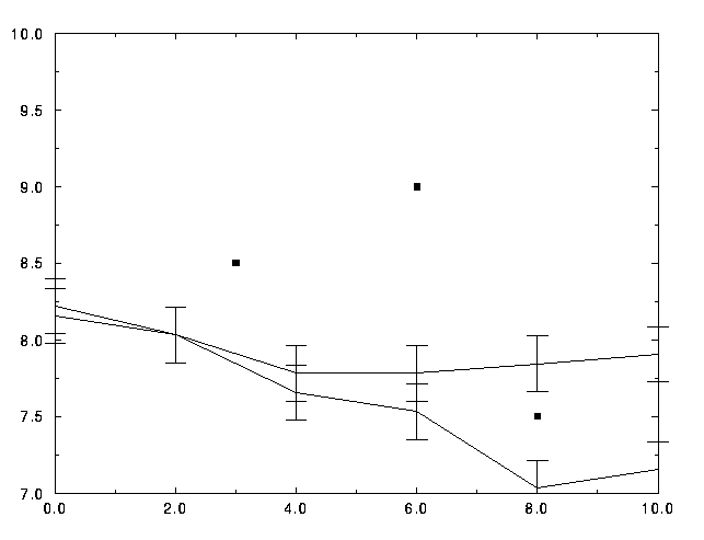
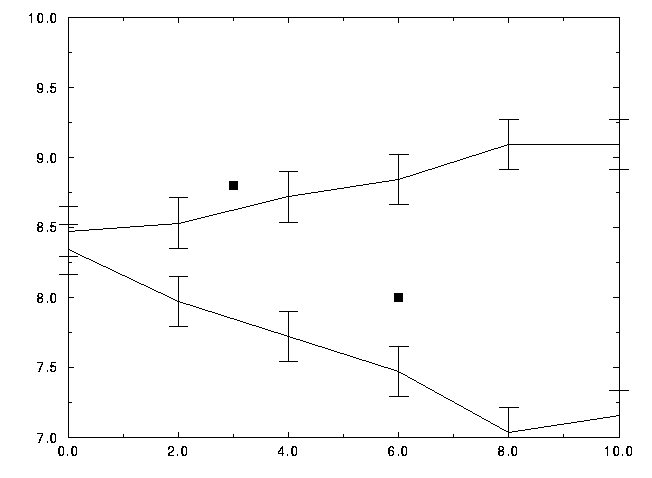
Figure 8 and 9 represent the transition lines in the plane  versus
the base 2 logarithm of
  in the case
of random initial distribution of purchasers and
of initial homogeneous half planes of purchasers.
The upper lines correspond to the lower
boundary of non-polluters domination. The
lower lines are the upper boundary of polluters partial domination
with a final market share larger than 0.8.
Since transients are very long in the neighborhood
of the transition, simulation times where restricted to 300 time steps.
Convergence towards polluters (resp. non-polluters)
domination was considered as certain
when the market share of polluters was above 0.8 (resp. below 0.1).
Although each transition point
is obtained by averaging over
nine simulations, the determination is not extremely precise,
due to the probabilistic character of information transmission.
Homogeneous initial conditions (figure 8) favors cooperation and the
choice of non-polluting cars with respect to random distribution
because the pollution gradient is large at the boundary
between the two regions, thus
giving a clear information to the agents in this neighborhood.
An interesting feature is the existence of an optimum memory range
( corresponding to a maximum difference in
prior utilities at the transition. This weak optimum was observed
consistently for all simulations. The agents performs better
by having an intermediate memory range, allowing them to
average information on several time steps while still
being able to cope with change.

Figure 8: Transition lines in the  ,
,  plane,
(the memory range scale is logarithmic), for
homogeneous half planes initial conditions as in figures
2, 3 and 4.
As in figure 8, the upper line is the lower
boundary of complete domination by non-polluters and the lower line
the upper boundary of mixed configurations with a market share of polluting
cars larger than 0.8. Pollution rate is 10. At low memory ranges,
the two transitions are simultaneous within simulation uncertainties.
Also note the slight minimum of
  as a function of
  around
  =32. The squares represent the parameters of simulation
for figures 2, 3 and 4.
When the agents are in a random environement (figure 9),
they have to rely
on pollution inhomogeneities to get useful informations.
The pollutions gradients are much smaller, which explains that
the upper transition line rests higher in  than for the homogeneous
initial distribution (figure 8).
Rather than averaging on several time steps to separate
signal from noise, they better follow time fluctuations
to get the meaningful signal: long term memory is thus a handicap,
hence the positive slope of the upper transition line.

Figure 9: Transition lines in the  ,
,  plane,
(the memory range scale is logarithmic), for
random initial distributions of polluters and non-polluters as in figures
6 and 7.
 the prior utility of polluting cars is set to 10,
and
  the prior utility of non-polluting cars varies
between 10 and 7.
The upper line is the lower
boundary of complete domination by non-polluters and the lower line
the upper boundary of mixed configurations with a market share of polluting
cars larger than 0.8. The upper transition is discontinuous, with market
shares of polluters varying from 0 to 0.75, while the lower transition
is continuous.
Pollution rate is 10. The squares represent the simulation
parameters of figures 6 and 7.
The lower transition lines are very similar for both kind of
initial conditions.
This systematic search of transition  when
when  is varied was also done for other pollution rates, s=20, and 5,
and give similar results, with the transition lines scaling in
 in proportion to s.


Next: CONCLUSIONS
Up: SIMULATION RESULTS
Previous: Description of some
weisbuch
Tue Feb 4 16:55:42 GMT+0100 1997
 versus
the base 2 logarithm of
  in the case
of random initial distribution of purchasers and
of initial homogeneous half planes of purchasers.
The upper lines correspond to the lower
boundary of non-polluters domination. The
lower lines are the upper boundary of polluters partial domination
with a final market share larger than 0.8.
Since transients are very long in the neighborhood
of the transition, simulation times where restricted to 300 time steps.
Convergence towards polluters (resp. non-polluters)
domination was considered as certain
when the market share of polluters was above 0.8 (resp. below 0.1).
Although each transition point
is obtained by averaging over
nine simulations, the determination is not extremely precise,
due to the probabilistic character of information transmission.
 corresponding to a maximum difference in
prior utilities at the transition. This weak optimum was observed
consistently for all simulations. The agents performs better
by having an intermediate memory range, allowing them to
average information on several time steps while still
being able to cope with change.

 ,
,  plane,
(the memory range scale is logarithmic), for
homogeneous half planes initial conditions as in figures
2, 3 and 4.
As in figure 8, the upper line is the lower
boundary of complete domination by non-polluters and the lower line
the upper boundary of mixed configurations with a market share of polluting
cars larger than 0.8. Pollution rate is 10. At low memory ranges,
the two transitions are simultaneous within simulation uncertainties.
Also note the slight minimum of
  as a function of
  around
  =32. The squares represent the parameters of simulation
for figures 2, 3 and 4.
 than for the homogeneous
initial distribution (figure 8).
Rather than averaging on several time steps to separate
signal from noise, they better follow time fluctuations
to get the meaningful signal: long term memory is thus a handicap,
hence the positive slope of the upper transition line.

 ,
,  plane,
(the memory range scale is logarithmic), for
random initial distributions of polluters and non-polluters as in figures
6 and 7.
 the prior utility of polluting cars is set to 10,
and
  the prior utility of non-polluting cars varies
between 10 and 7.
The upper line is the lower
boundary of complete domination by non-polluters and the lower line
the upper boundary of mixed configurations with a market share of polluting
cars larger than 0.8. The upper transition is discontinuous, with market
shares of polluters varying from 0 to 0.75, while the lower transition
is continuous.
Pollution rate is 10. The squares represent the simulation
parameters of figures 6 and 7.
 when
when  is varied was also done for other pollution rates, s=20, and 5,
and give similar results, with the transition lines scaling in
 in proportion to s.