Alexandros ALEXAKIS
CNRS, Département de Physique, Ecole Normale Supérieure (ENS Paris)
CNRS, Département de Physique, Ecole Normale Supérieure (ENS Paris)
Research
|
|
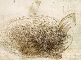
TurbulenceThe root of all trouble. Turbulence, the last problem of classical physics, has been around for a long time. The figure on the left, drawn by Leonardo Da Vinci, gives one of the first descriptions of turbulence [not to mention Greek philosophers :) ] that seems to include the ideas of a cascade. Although, physical processes that are involved seem to be understood: eddies being self-stretched generating smaller eddies that are themselves stretched and so on until dissipation scales are reached, we do not seem to be able to give a precise (rigorous hopefully) prediction for different statistical properties of a turbulent flow. Andrey Nikolaevich Kolmogorov in 1941 (K41) gave the first quantitative description of turbulence. Typically Kolmogorov's 1941 arguments are presented in terms of dimensional analysis and predict that the moments of velocity differences scale likeMy own interests also lie in the origin of intermittency, the behavior of small scales as well as the behavior of global quantities like the energy dissipation rate. [[Publications : 11,13,14] |
|
|
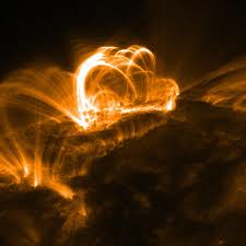
(MHD) Magneto-Hydro-Dynamic TurbulenceThe root of all my trouble. MHD-Turbulence involves the largest part of my work. The solar flares shown on the left are an example of an MHD turbulent flow. Unlike Hydrodynamic (HD) turbulence in MHD we have not yet reached even the K41 level. There are still debates in the literature whether the energy spectrum (or equivalently the second velocity-difference moment) has an exponent -5/3 of K41 or -3/2 predicted by Iroshnikov and Kraichnan (IK). It is also not clear if the exponent has a unique value, thus the assumption of universality could be questioned. One of our biggest difficulties in MHD turbulence is that unlike HD that everything is controlled by one number (ie Re) in MHD we have a lot more to worry about. To begin with we have two non-dimensional numbers Re and Rm each expressing the ratio of non-linearities to dissipation mechanisms (viscous and Ohmic). We can not a priori assume that the regimes Re>>Rm, Re~Rm and Rm>>Re have the same statistics even if we are looking at scales that both dissipation mechanisms are very small. We also expect that flows with more kinetic energy than magnetic energy will behave differently from flows with more magnetic energy than kinetic energy (weak turbulence). Furthermore we have to distinguish between flows with helicity (Helical turbulence) that have an inverse cascade from flows without helicity. [Helicity is an ideal invariant measuring the knoted-ness of the field lines]. Flows with large cross helicity (imbalanced turbulence) or without cross helicity also result in different behavior. [cross-helicity is an ideal invariant measuring the correlation between the two fields u and b]. Thus MHD pose a much more rich problem than HD turbulence. The question that interests me is how to model the energy cascade in MHD turbulence, in all these different regimes. My studies of the locality of interactions in MHD turbulence showed that in comparison with HD turbulence they appear to be more nonlocal. In the presence of a mean magnetic field the cascade also becomes anisotropic and thus forming a complex wide range network of interactions between different scales. How this behavior can be modeled? are the results universal? in what sense? are some of the questions I am interested in.[[Publications : 3,4,10,12,14,17-19,29,32,34-36,41] |
|
|
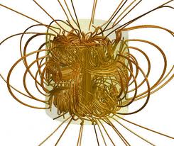
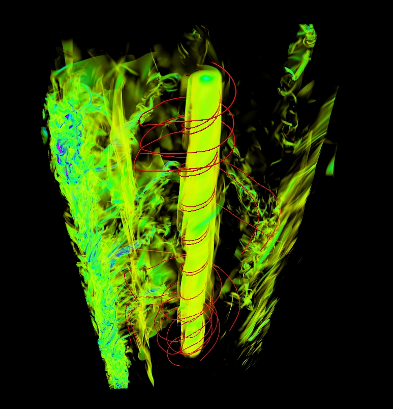
Magnetic DynamoTrouble that grows! The magnetic dynamo theory is in principle part of the MHD turbulence problem, however it exhibits such richness of behavior that it deserves its own paragraph in this webpage. The figure on the left has been taken with out any shame from the work of Christophe Gissinger and shows the magnetic field lines generated by a dynamo flow in a cylindrical container. The flow is a model for the VKS dynamo experiment that my group is involved with. The dynamo problem can be split in two parts exponential growth and saturation. For (infinitesimally) small magnetic energy the evolution equation for magnetic field is linear, thus (in a finite domain) after a transient regime magnetic energy is expected to increase or decrease exponentially. And the question is: with what growth rate? In addition we can ask what are the properties of the growing field (small scale vs large scale)? what are the properties of the velocity field needed to achieve dynamo? The linearity of the problem allows us to examine such properties in much greater detail than a non-linear problem. In the nonlinear (saturated) stage we reach a special case of MHD turbulence. How at what amplitude and at what scale the magnetic field saturates is a very open question in dynamo theory. The answer to these questions is not simple neither unique. The saturation amplitude of the magnetic energy has been found to be orders of magnitude smaller or bigger than the kinetic energy depending on the type of flow and the value of the kinetic and magnetic Reynolds number. My work on dynamo wanders about special cases like the infinite Prandtl limit, or close to onset (on-off intermittency) where more detailed investigations can be made.[[Publications : 9,15,21,22,276,27] |
|
|
MixingIf we can not understand this what hope do we have for dynamo? The advection-diffusion equation is perhaps the simplest PDE model of a cascade in scale space. Despite its simplicity it can result in a rich behavior if the velocity field that moves around the scalar is sufficiently complex. It shares many common properties with the linear dynamo problem and thus my interest in the problem. The figure on the left shows the classical stretch-and-fold structures of an advected scalar. It was obtained from a numerical simulation of the advection-diffusion equation in the presence of sources and sinks. The behavior of the system however can be much more different than this if the injection scale is different than the advection scale. My recent work with Alexandra Tzella investigated the case when scalar field was introduced at one scale while stirred at an other. The interplay between transport, stirring and diffusion lead to the prediction of 5 different regimes of mixing with different scaling behavior for each. Non-linearity can also be included in this problem if one considers a reaction term, this is typical for the study of chemical reactions, plangton and bacteria evolution, etc. Although I find that exciting I have not ventured in that path yet.[[Publications : 28] |
|
|
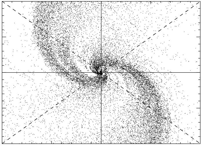
Inverse cascadesTurbulence in flatland and beyond. Turbulence does not always generate a mess. In some cases it can self-organize to generate large scale structures through a process known as an inverse cascade. The simplest example probably is turbulence in two dimensions (2D). In 2D eddies self-interact to generate larger eddies and so on and energy instead of cascading in the small scales (as in 3D turbulence) it cascades inversely in the large scales where it piles up. There are some examples, however, that have a mixed behavior such as fast rotating fluids, conducting fluids in the presence of strong magnetic fields, flows in constrained geometry, and others. In these examples the injected energy cascades both forward and inversely in fractions that depend on the value of a control parameter (rotation rate/magnetic field/aspect ratio etc). In our work we have demonstrated by studying 2D-MHD that the transition from a forward to an inverse cascade can be through a critical point. Close to this point the energy flux scales as a power law with the departure from the critical point and the normalized amplitude of the fluctuations diverges. The figure on the left shows the vorticity of a flow in a 2D-MHD simulation where both forward and inverse cascades exist.[[Publications : 12,14,29,39,40] |

|
|
Rotating FlowsAn other example of waves an turbulence. The figure on the left shows the vorticity density of a flow with a relatively strong rotation rate. It was obtained by a numerical simulation of carried out by Pablo Mininni. In this figure both columnary (2D) and three dimensional structures are visible. Like MHD a rotating flow is a system that supports both eddies and waves. Also, like MHD with a strong magnetic field, strong rotation makes the system quasi-two-dimensional where most of the energy is in the 2-D component but the smaller 3-D component can not be neglected since it breaks the conservation of vorticity. Unlike the MHD however there is only one field involved thus making the problem more tractable analytically and numerically.[[Publications : 23,40] |
|
|
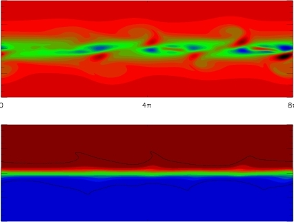
Stratified FlowsMore waves and more turbulence. This a third example of a system where both waves and eddies live. However the properties of the flow in the limit of strong stratification can be very different than that of strong rotation or strong magnetic field. The previous examples do not favor variation along the direction of wave-propagation thus the flow becomes quasi-2D. In the strong stratification limit waves propagate more strongly in the horizontal plane and thus variations along the the vertical direction are preferred. My work on stratified flows is limited in the studies of Holmboe instabilities. Holmboe instability (also known as the cousin of Kelvin-Helmholtz instability) appears in stratified shear layers whose variation length scale is much larger than that of the stratification. It results in propagating gravity waves whose breaking cusps result in to upwards mixing. My work revealed that there is an infinity of such modes of increasing complexity that appear at larger values of stratification. The figure on the left shows such a wave formed a global Richardson number equal to 20. The top figure is a color-scale plot of the vorticity field while the figure on the bottom is a color scale picture of the density field. Although the global Richardson number (a measure of the strength of stratification) is so large locally it can be small and these regions allow the instability to develop.[[Publications : 1,2,5-8,16,24] |
|
|
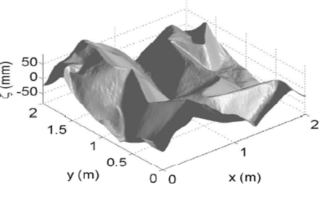
Elastic wave turbulenceMore waves, more turbulence but no flow. The phenomenon of turbulence is not restricted only in flows. The same principles govern all (out of equilibrium) non-linear systems with many degrees of freedom where energy is injected in one scale and dissipated at an other. Non-linear waves on an elastic plate is such an example. The figure on the left shows the distortion of an elastic plate by strongly forced elastic waves. It is a result from a numerical simulation of the Foppl-Von Karman equations that govern the evolution of the deformations of a plate. Strong cusps appear that are related to crumpling phenomena. This work was done in collaboration with Nicolas Mordant and Benjamin Miquel that also performed laboratory experiments.[[Publications : 33,38] |
|
|
ModelsJust because we can not solve the ones before. The answer to the following question is my objective for any kind of modeling. Given an observed phenomenon what is the minimum number of "ingredients" one needs to include in a model to reproduce the phenomenon. If this is achieved then I think we have began to understand what the phenomenon is all about. In this respect a successful model can be more useful than a brute-force numerical solution. With this goal in mind there is number of phenomena that are observed in non-linear physics that require this kind of modeling to be understood, and many different approaches to modeling that can be applied. Low-order-models, stochastic-modeling, shell-models, ODT, simple maps, are some of the models that have caught my attention at various times.[[Publications : 18,25,30,31] |