

Next: Algebraic analysis
Up: Prices
Previous: Prices
Economists have raised strong objections
about the dire outcomes predicted by envionmentalists
using systems dynamics models,
such as that of the Club of Rome [Meadows  , 1972].
One of their criticisms concerns the ability
of market mechanisms to damp dangerous oscillations [Stiglitz, 1979,Cropper
  , 1979]. The argument is
that when a resource becomes rare
its concomitant price increase
lowers its exploitation, or favors technologies
less wasteful in resource usage.
Let us rewrite the production in monetary units as

where

in order to introduce a production in value which depends upon the production
in fishes, instead of the previous expression which
contained only a constant production coefficient,  .
.
The differential equation for the resource, N,
remains unchanged.
(We use equation 3 from section 2 without the
carrying capacity term).
The only change occurs in the differential equation for the
capital:

A simple monetary coefficient function  is given by:

and the differential equation for the capital is then:


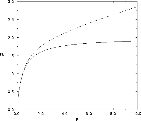
Figure 8: Plot of the production expressed in monetary units,  ,
as a function of production, P, for the
functions used in section 4. The solid line corresponds
to "market" prices with coefficients b=2 and
  of the first model, equation 33.
Note the plateau region which gives
a constant income at large production. The dotted line
corresponds to the second model with a minimum sustained price
 , with the same values for b and c, equation
39.
Figure 8 indicates a simple interpretation of the
coefficients
b and c in the fraction  : b is a maximum production in value, obtained when the catch
goes to infinity, and c is a characteristic scale on the production P.
 is the maximum price, which is obtained at zero production.
We might consider that the above function reflects
the situation where there is a
strong decrease of prices with production since value production
saturates at high production: there remains no incentive
for producers to increase the catch in this regime.
Under "normal"
circumstances, the decrease of
  with P is probably
less strong than in expression 33. Price dynamics under
normal economic conditions
are probably intermediate between the models of section 2 and 4.


Next: Algebraic analysis
Up: Prices
Previous: Prices
weisbuch
Fri Feb 7 13:18:37 GMT+0100 1997
 , 1972].
One of their criticisms concerns the ability
of market mechanisms to damp dangerous oscillations [Stiglitz, 1979,Cropper
  , 1979]. The argument is
that when a resource becomes rare
its concomitant price increase
lowers its exploitation, or favors technologies
less wasteful in resource usage.


 .
.

 is given by:


 ,
as a function of production, P, for the
functions used in section 4. The solid line corresponds
to "market" prices with coefficients b=2 and
  of the first model, equation
  , with the same values for b and c, equation
 : b is a maximum production in value, obtained when the catch
goes to infinity, and c is a characteristic scale on the production P.
 is the maximum price, which is obtained at zero production.
We might consider that the above function reflects
the situation where there is a
strong decrease of prices with production since value production
saturates at high production: there remains no incentive
for producers to increase the catch in this regime.
Under "normal"
circumstances, the decrease of
  with P is probably
less strong than in expression