The equilibrium resource level  is obtained by equating the left-hand side
of equation 34 to zero:
is obtained by equating the left-hand side
of equation 34 to zero:
A positive resource equilibrium is only achieved when the
maximum production b is larger than the capital depreciation rate during
the same period,  , otherwise the capital keeps on decaying.
The equilibrium resource gets bigger and bigger as
the maximum production in money gets closer to the capital depreciation
per unit time.
, otherwise the capital keeps on decaying.
The equilibrium resource gets bigger and bigger as
the maximum production in money gets closer to the capital depreciation
per unit time.
Now that both  and
and  are known
the stability analysis can be done around
the equilibrium.
are known
the stability analysis can be done around
the equilibrium.
The following expression is obtained for the stability parameter
 :
:
where  . Note that the dynamical behavior
only depends upon
. Note that the dynamical behavior
only depends upon  and
and  , but not on c.
Damping of oscillations, related to the real part
of  , is increased by prices by a factor
Prices do attenuate the oscillations, and thus resource depletion, but since the fraction should be smaller than one for equilibrium to exist, the damping factor is at most 2.
The region of oscillation is decreased by prices. Oscillations occur when
In fact expression 33 refers to a situation when demand is large
and when prices are adjusted by classical supply demand adjustment
mechanisms. This is generally the case for artisanal fisheries
of highly valued species such as sole, cod, haddock,
shrimps and lobsters.
But for some fisheries, such as french industrial fisheries of
hake , herring, anchovy, market demand can be low with respect to production.
In this context, in order to preserve the economic fishing sector,
landing prices are maintained by institutions such as government or producer
organizations.
We can further complicate the monetary coefficient function  by introducing a minimum price a for fish (see figure 8),
to model the case of a minimum price maintained by some institution:
by introducing a minimum price a for fish (see figure 8),
to model the case of a minimum price maintained by some institution:
A full algebraic analysis of this system, reported in the Appendix,
has been done which gives expressions
which are difficult to interpret;
but we can still predict the two extreme dynamical regimes.
When the minimum price is
low, the major difference is that the restriction on b no longer
holds since a production equilibrium always exists.
At low equilibrium production the minimum
price can be neglected
and the above analysis (beginning of this section)
makes it possible to predict the dynamics. In the large production region
the standard analysis of section 2 applies with  as if the price
were simply
as if the price
were simply  . Large resource depletion is observed,
and the equilibrium resource is maintained at a level
inversely proportional to a.
. Large resource depletion is observed,
and the equilibrium resource is maintained at a level
inversely proportional to a.
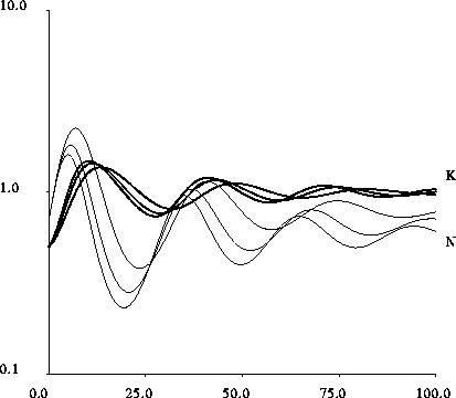
Figure 9: Time plot of the resource population and
capital for the model of section 4,
which takes into account the role of prices.
Prices damp the oscillations, but the effect is lessened by the existence
of a minimum price. The parameters of equation 39
are b=2 and c=0.5, corresponding to a maximum price of 4,
and a minimum price of 0.1 (for the most damped oscillation), 1
and 2 (for the biggest oscillations).


