 equilibrium, which existed for all previous models, is no longer a possible equilibrium state since some level of consumption still occurs
even when there
are no fish and no boats.
Equilibria:
There is only a single equilibrium for this new system. The  equilibrium, which existed for all previous models, is no longer a possible equilibrium state since some level of consumption still occurs
even when there
are no fish and no boats.
Normalizing N and
K with respect to the  and
and  of section 2,
the equilibrium with the new consumption function is at
 =
=  , where
The positive equilibrium is at the same capital
level as before, but the equilibrium number of fish
is larger than the baseline value of  .
Clearly this occurs because more of the capital is drained off into consumption
and less can be used for harvesting fish. The equilibrium level
of the resource,
  , increases with the minimum consumption,
  ,
the width of the transition region
(as governed by
  ), and the fraction of profits are that are consumed,
  .
.
Substituting the equilibrium values of the resource and the capital back
into the expression for  shows that the consumption at the equilibrium
point is equal to
  , or
, or  . Thus when the
corner in the consumption function becomes sharp, (
 ), the equilibrium is at the corner, with
  .
.
Stability:
When the equilibrium point lies near the region of minimum consumption, it is strongly modified by the existence of this minimum consumption. We can still have a stable equilibrium with oscillations, but the size of the parameter region where oscillations do occur is different, and for some parameter values the equilibrium is no longer stable.
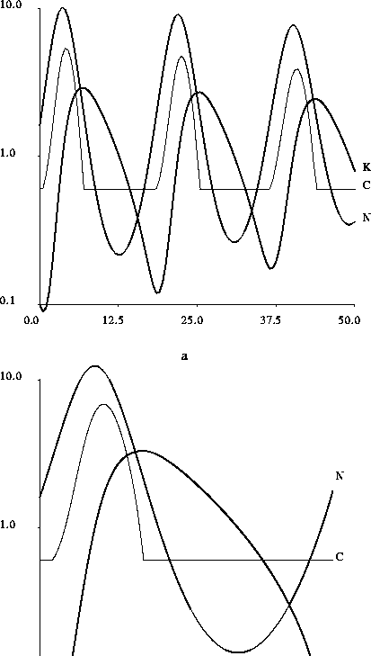
In addition, a positive minimum consumption implies that the derivative of K is negative at K=0: when the initial capital is small, the system might collapse even though the equilibrium is attractive (see figure 11b).
Linearizing the system around the equilibrium gives the eigenvalues
where

Figure 11: Time plots of the logarithms of
resource, capital, and consumption for the model of section 5. Here N and K are scaled by  and
and  , respectively, of section 2, and the consumption C is scaled by
  . Shown are two different initial conditions for the case
  ,
,  = 0.5,
  , and
, and  . In both cases N starts out at its equilibrium value of
  . Each time the profit plummets to
  or less,
the consumption bottoms out to
  .
(a)
.
(a)  . In this case the initial conditions are in the attracting region of the equilibrium, and capital never
goes to zero.
(b)
  . Although this initial condition is near to that of (a), it is just outside the zone of attraction of the equilibrium. The amplitude of the oscillations gradually grows, until capital collapses.
The equilibrium is thus stable as long as  ,
i.e. when equilibrium resource level is lower than twice
harvesting equilibrium.
For very small values of
  this condition is equivalent to
  .
When
  cannot be neglected the transition occurs
for smaller values of
  .
As
.
As  increases, the real part of
  goes to zero, and
attraction gets gradually weaker.
However, even before
  reaches 2,
an unstable region can occur, and trajectories can hit the boundary if the capital gets too small (figure 11b).
In fact the basin of attraction of equilibrium shrinks
in the phase space as
  increases.