 , 1992,Meadows
  , 1972].
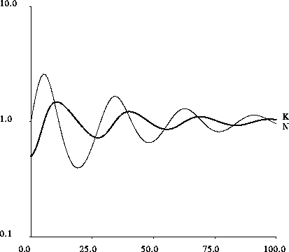
Figure 2 displays the capital and the resource as they vary with time.
Solutions are damped oscillations which gradually converge to an equilibrium
point.
Note that when the initial conditions are not near equilibrium
the first oscillation is quite strong: this corresponds to a
real depletion of the resource, which would have a dramatic
impact on the income level of labour. The present paper focuses
on this effect. Of course one might
imagine other initial conditions, but there is no reason to
suppose that resource exploitation starts
anywhere close to a production equilibrium.
Instead, for previously unexploited or lightly exploited resources,
the resource
usually starts at some high level and capital starts from a low value
since it has not had sufficient time to accumulate.
The large overshoot in capital observed in figure 2,
followed by extreme resource depletion, corresponds to the most
dramatic scenarios described, for example, in Beyond the Limits (p. 108) [Meadows  , 1992,Meadows
  , 1972].

Figure 2: Logarithmic plot of the time variations of the normalized capital,  ,
and the normalized resource,
  , for the
simple model of section 2. Normalized variables and parameters
are discussed in section 2.3. Time is scaled in units of
  ,
and this scaling is the same
for all time plots.
Initially the resource is at equilibrium (
 ), while the capital
is at one half of the equilibrium (
 ). Here
  .
Note the strong resource depletion during the first oscillation, even though initial conditions are not far from equilibrium.
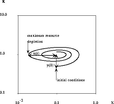
One of the purposes of the present paper is to study the magnitude of this resource depletion under the influence of a number of mechanisms which were supposedly absent from the Limits to Growth model, such as technological improvements, prices, and dynamics of consumption...and compare how much each mechanism reduces the level of resource depletion. Resource depletion is systematically measured, using numerical simulations, as a function of the fraction of initial capital with respect to the final equilibrium capital, with the initial resource being taken to be its equilibrium value (see figures 3, 6 and 14). Resource depletion can also be analytically computed in the neighborhood of the equilibrium point using the linear approximation. This is done in section 2.3.

Figure 3: Trajectory in the phase plane showing the initial conditions,
with a relative deviation y(0) of the capital from its equilibrium value,
and the point of maximum relative resource depletion, x(t), used in figures 6 and 14 diagrams.