 and
and  , where
This system has a nontrivial equilibrium state, given
by  and
and  , where
In the rest of this paper the algebra and simulations
will be performed with non-dimensionalized systems.
Nondimensionalizing the system, by changing variables, reduces the
number of parameters in the system and allows us to examine all at
once a set of parameters which lead to the same mathematical behavior.
For example, as we will
see, all parameter choices
with the same values of  yield the
same dynamical behavior, no matter what r,
  and
and  are.
In order to interpret results, we will sometimes come back to the original
variables and parameters.
We use the equilibrium values of N and K, and the rate of resource replenishment r, to nondimensionalize the system by letting
This gives the nondimensionalized system:
with only one parameter remaining:
 gives a measure of the ratio between the rate of decay of capital and
the replenishment rate of the resources.
This system has two
equilibria at  = (0, 0) and (1, 1).
The equilibrium around the origin is unstable.
Linearizing around the point (1,1) gives:
which has eigenvalues  .
This equilibrium is always stable. If
  this equilibrium is
reached without oscillations.
If
  oscillations decay toward the
equilibrium. The magnitude of the oscillations of course depends on
the initial conditions, being larger the further the initial system is from equilibrium (figures 6 and 14).
These oscillations are
the dramatic oscillations that are observed by numerical simulations
in figure 2 for instance. In the limit of small
  , the oscillation frequency is:
where the r factor comes from changing back the time scale from  to t.
to t.
Resource depletion as a function of the distance of the initial conditions
from equilibrium can also
be estimated
analytically, at least when solutions are so close to equilibrium
that
the linear approximation is valid.
Figure 3 shows that we have to relate  , the
relative resource
depletion at time t,
where t is the time for the system to rotate
  around equilibrium,
to
  , the initial relative deviation of capital from equilibrium
(relative here refers for instance to the ratio of initial
capital to capital at equilibrium).
where  and
and  are the real and imaginary part of
 . The ratio of
  and
and  is obtained from equation 11,
where the time derivative of x is replaced by
  .
.
We can then define the linear fragility f of any bio-economic system with overshoot and depletion by:
which gives:
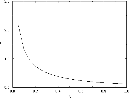
for system 3-4. High fragility refers to a strong resource depletion following any initial departure for equilibrium. Linear fragility
can a priori take any value between 0 and infinity. The variations
of f with  are represented on figure 4.

Figure 4: Linear fragility, defined in the text as the ratio
between maximum relative resource depletion to initial relative capital
distance to equilibrium ( see figure 3)
is represented as a function of  defined by equation 9. Computation is done
according to equation 17. The fragility of the
system increases when the renewal rate of the resource is
much faster than capital depreciation rate.